Jev and System One models: typed decisions

Artificial Intelligence

EU AI Act consulting: system classification, policies, AI governance, training.

Discover →

Cybersecurity

CISO-as-a-service consulting: posture, remediation roadmap, ongoing support.

Discover →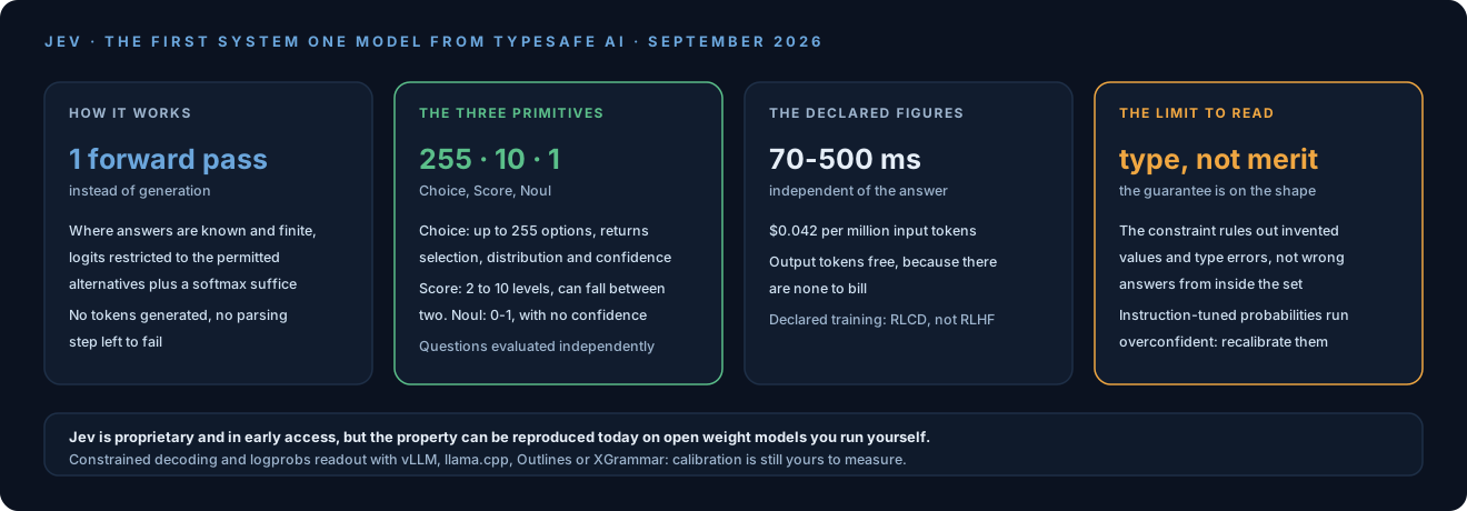

TypeSafe AI has opened access to Jev, which the company presents as the first System One model. The company was founded by Diogo Almeida, who comes from OpenAI. The model is in early access behind a waitlist, proprietary and reachable through a hosted API.

The name comes from Kahneman, and the documentation says so: “The System One name comes from the concept Daniel Kahneman popularized in his book Thinking, Fast and Slow”, where system 1 is fast, intuitive thinking. It is a label TypeSafe chose for its own product rather than a category the industry already shares.

The way TypeSafe describes it is unusual and worth taking literally: Jev gives up string generation. It does not produce text. It takes a state and typed questions, and returns structured values with a probability distribution over them.

This article explains the principle, shows what the endpoint is and how a request is built, and then shows how to get an analogous property from open weight models you can run yourself.

What machine learning has always known

Before the mechanism, it is worth saying something that will sound very familiar to anyone who worked with machine learning before language models, ourselves included.

A classifier has always done exactly this. You define the set of classes, you train the model on them, and the last layer returns a probability distribution over that set. There was no parsing step because there was no text to interpret, and the output was already a number per permitted class.

Calibration is an old subject too. Reliability diagrams, Platt scaling and temperature scaling have been in the textbooks since long before this season, and the literature on overconfident deep networks is almost ten years old. Anyone who has put a classifier into production for diagnostic support, for routing or for quality control has had to look at that curve before fixing a threshold, because that is where you decide when the machine acts on its own.

Then there is the economics, which weighs a good deal over time. On a narrow task, with a stable taxonomy and representative labelled data, a specialised classifier can be cheaper and also more accurate than a general model. It is not a guarantee, and that is worth saying: the advantage depends on data quality, input coverage, how often drift happens and the cost of maintenance. Where the advantage does exist, it shows up on three lines. Training is often measured in hours on a single card. Inference is one pass over a small model, which in many cases runs on CPU too, depending on size, latency and volume. And retraining stays a repeatable operation: the taxonomy changes or the distribution drifts, so you relabel, retrain and compare the metric against the previous one.

That last point is the most underrated. With a classifier, retraining comes with a number that says whether it got better or worse. A prompt-based system can have the same discipline, with an evaluation suite and regression tests over the answers: the trouble is that in practice this test bench often does not get built, and then the regression surfaces in production.

What changed in recent years is the interface. Language models made text the universal channel, and with text came the habit of asking for a classification inside a prompt, getting it back as JSON and recovering a value from it with a parser. The general-model route remains the only possible one where labelled data does not exist, where the answer set keeps changing, or where the task needs world knowledge a locally trained classifier does not have. Where the set is known and the data exists, it is a detour around a problem the discipline had already solved another way, and at a different cost.

Seen like this, the novelty of a model like Jev is less a break than a call back to a method: you choose which answers are permitted first, you measure how reliable the model is on those, and you read the number. It is also why the useful part of this release applies without Jev, and takes up half of this article.

Why TypeSafe declares lower latency

The principle is simple and worth isolating, because it explains the shape of the figures that follow.

An LLM generates text one token at a time. To get a structured decision out of one you write a prompt asking for JSON, the model generates those tokens one after another and the calling code parses and validates what came back. Latency depends on how long the output is, and the parsing step can fail.

Where the alternatives are finite, though, a system need not produce a textual answer token by token: it can compute scores or probabilities over the permitted options directly. That is the technique behind the open weight half of this article, where you run a forward pass, look at the logits restricted to the alternatives and apply a softmax.

On Jev itself, it is worth being precise about what is known. TypeSafe declares a new architecture with a hardware-aware parallel sampler that returns the decisions in parallel. The public material does not describe the model in enough detail to reduce it to an ordinary LLM whose logits are read in a single forward pass: that is a possible technique, used by some of the open implementations, rather than a verified description of Jev.

The figures are the vendor’s. TypeSafe declares end-to-end latency between 70 and 500 ms, $0.042 per million input tokens and no separate price for output tokens. These are measurements and commercial terms published by the party selling the service, to be checked against the load, region and model version you actually use.

The phrase “latency does not depend on the answer” also needs care. It does not grow autoregressively with the length of a generated string, which is the point. It can still depend on the length of the state, the number of questions, the cardinality of the options, batching and service load. On high-cardinality choices TypeSafe says so itself in a note to the launch post: “For the higher cardinality choices, we do a 2 stage-system of scoring independently then making an explicit choice, hence the occassional slowdown”.

TypeSafe adds a piece of its own on training: instead of RLHF it says it uses RLCD, Reinforcement Learning for Calibrated Decisions, optimised to produce honest probabilities rather than answers a human rater likes. We come back to this at the end, because it is the difference that matters.

The three primitives

Each request evaluates one state against one or more questions. All questions see the same state and are evaluated independently: adding or removing one does not change the answers to the others.

Choice. A selection among options with no order between them. You pass criteria as a map from option to description. It accepts up to 255 options. It returns choice with the selected option, probabilities with the distribution across every option, and confidence.

On Choice there is a recommendation in the documentation always worth following: where the taxonomy might not cover every input, add an other or none of the above option, “so the model can say none of the others fit”. Without a way out the model has to pick even for an input that belongs to no class, and a very concentrated distribution across forced options does not show that any of them fits.

Score. A position on an ordered scale. You pass criteria as an ordered array of level descriptions, from at least 2 up to 10. It returns score, which can fall between two levels (in the documentation’s example it is 1.035), plus legend, probabilities and confidence.

Noul. A yes/no question where the interesting number is the probability itself. It returns only noul, a value between 0 and 1. It has no confidence, and the documentation warns that 0.5 means the model gives yes and no equal probability rather than that the quantity being measured sits halfway.

On that last point the documentation is explicit, with a useful example: “Is this candidate strong in Python?” is a badly posed Noul, because “strong” is not defined. To measure a level you want a Score with the levels written out; for a binary decision you want a sharp condition, such as “does the resume state that the candidate has used Python at work?”.

The first call

There is a single endpoint.

POST https://api.typesafe.ai/v1/systemone
Authorization: Bearer <API_KEY>
Content-Type: application/json

The body has three top-level fields: state, model and questions. Here is a request asking all three question types at once about a support ticket.

{
  "state": "Hi, I've been trying to connect my Stripe account for 3 days and it keeps failing. I'm losing sales. Please help ASAP.",
  "model": "jev-latest",
  "questions": {
    "department": {
      "type": "choice",
      "instructions": "Which team should handle this",
      "criteria": {
        "billing": "Payment or subscription issues",
        "technical": "Bugs or integration problems",
        "sales": "Pricing or account questions"
      }
    },
    "frustration": {
      "type": "score",
      "instructions": "How frustrated the customer appears",
      "criteria": [
        "Calm, just stating facts",
        "Frustrated but civil",
        "Very angry, strong language"
      ]
    },
    "is_urgent": {
      "type": "noul",
      "instructions": "The message conveys urgency or time-sensitivity"
    }
  }
}

The response carries all three evaluations in one go. The example is taken from the Quick Start documentation, and comes with a caveat: the primitives page lists probabilities among the Score fields too, while this example does not show them, so the actual payload needs checking against the API version you use.

{
  "model": "jev-latest",
  "answers": {
    "department": {
      "type": "choice",
      "choice": "billing",
      "probabilities": { "billing": 0.84, "technical": 0.159, "sales": 0.001 },
      "confidence": 0.596
    },
    "frustration": {
      "type": "score",
      "score": 1.035,
      "legend": { "0": "Calm, just stating facts", "1": "Frustrated but civil", "2": "Very angry, strong language" },
      "confidence": 0.842
    },
    "is_urgent": { "type": "noul", "noul": 0.999 }
  },
  "usage": { "input_tokens": 312, "output_tokens": 48 }
}

This response repays a careful look, because it carries a lesson. The model picks billing with a probability of 0.84, while confidence is 0.596: two different numbers measuring different things. The threshold above which to automate cannot be deduced from this single case; it has to be chosen against the risk and validated on labelled data from your own domain. A score of 1.035 places the customer just above the “frustrated but civil” level, because the score can fall between two levels.

One more thing visible in the payload: output_tokens is 48. The output count exists and is reported, while what TypeSafe claims is the absence of autoregressive generation and a commercial price of zero for that line. Those are three distinct statements and it is worth not conflating them.

The state need not be a string: it also accepts JSON objects and arrays, and that is the form to prefer when the context has distinct named parts. Jev accepts text only, no images, audio or video, and its primary training language is English: the documentation warns that other languages are accepted with lower accuracy. For a ticket in Italian, measure before trusting.

The Python SDK

It needs Python 3.10 or later. The client reads the key from TYPESAFE_API_KEY and calls jev-latest by default.

pip install typesafe-sdk

from typesafe_sdk import Choice, Noul, Score, TypeSafeClient

state = {
    "ticket_message": (
        "Hi, I've been trying to connect my Stripe account for 3 days "
        "and it keeps failing. I'm losing sales. Please help ASAP."
    )
}

client = TypeSafeClient()

response = client.system_one(
    state=state,
    questions={
        "department": Choice(
            instructions="Which team should handle this",
            criteria={
                "billing": "Payment or subscription issues",
                "technical": "Bugs or integration problems",
                "sales": "Pricing or account questions",
            },
        ),
        "frustration": Score(
            instructions="How frustrated the customer appears",
            criteria=["Calm, just stating facts", "Frustrated but civil", "Very angry, strong language"],
        ),
        "is_urgent": Noul(instructions="The message conveys urgency or time-sensitivity"),
    },
)

print(response.answers["department"].choice)   # "billing"
print(response.answers["frustration"].score)   # 1.035
print(response.answers["is_urgent"].noul)      # 0.999

How to use confidence

This is the part that genuinely changes the code you write, and it does not require Jev to be applied.

confidence is a statistic computed from the shape of probabilities: a distribution concentrated on one option gives high confidence, a flat one gives low confidence. It should be read for what it is. A confidence of 0.596 does not mean the choice has a 59.6% chance of being right: it is a concentration index defined by the vendor. The probability of the top option, the confidence and the empirical accuracy are three different quantities, and only the third is measured on labelled data.

The documentation says so plainly and adds an honest point, namely that their definition is a convenient default and that they return the whole distribution precisely so you can compute the measure you need.

The suggested pattern splits into three bands and mirrors what a serious system does anyway:

• High confidence: act automatically.
• Medium confidence: proceed with caution, asking the user to confirm or flagging the case for review.
• Low confidence: do not act, and route to a person.

A real design also needs the things that number cannot see. An input out of distribution, or one simply missing the necessary information, can produce a concentrated and wrong distribution, so alongside the thresholds you want an explicit abstention option, a human fallback path, different thresholds for reversible and irreversible actions and drift monitoring that tells you when yesterday’s calibration no longer holds.

The value of this scheme sits in one line of the documentation that holds regardless of vendor: a system that cannot express honest uncertainty is not a system you can rely on. It is the same principle we keep coming back to in the anatomy of an agentic loop: the threshold that decides when to stop is written beforehand, not inferred afterwards.

How to reproduce it with open weights

Jev is proprietary, hosted and behind a waitlist. The property of constraining output to finite alternatives, though, is not exclusive to Jev and can be implemented with open source tools, on models you run yourself. It is worth being clear about what reproduces easily and what does not.

The constraint on the shape can be had in several ways, all open source and all mature.

With vLLM you use structured outputs. Mind the version, because the API changed: the old guided_* fields were removed in vLLM 0.12.0 and replaced by structured_outputs. The snippet below is the one documented for vLLM 0.12 and later and still needs checking against the version you have installed.

from vllm import LLM, SamplingParams
from vllm.sampling_params import StructuredOutputsParams

llm = LLM(model="Qwen/Qwen3-8B")

structured = StructuredOutputsParams(choice=["billing", "technical", "sales"])
params = SamplingParams(structured_outputs=structured)

out = llm.generate(prompt, params)
print(out[0].outputs[0].text)

This block guarantees the shape of the output: the text produced will be one of the three labels. It does not by itself return the distribution over the alternatives, which is a separate and more delicate problem.

With llama.cpp you get the same through a GBNF grammar, which describes the permitted shape and enforces it during decoding:

root ::= "billing" | "technical" | "sales"

There are also Outlines and XGrammar, the latter used as the structured generation engine inside vLLM and SGLang.

The distribution, the part that makes the answer usable as a signal rather than only as a label, comes from the logprobs, normalised over the permitted alternatives alone. Here is the formula, written as a conceptual sketch rather than a runnable example, because how you obtain those values differs from engine to engine.

import math

# lp_* are the logprobs of the tokens identifying the options.
# How to retrieve them depends on the engine: on vLLM through
# logprobs or prompt_logprobs, on Transformers from the step logits.
cand = {"billing": lp_billing, "technical": lp_technical, "sales": lp_sales}
z = sum(math.exp(v) for v in cand.values())
probs = {k: math.exp(v) / z for k, v in cand.items()}

# Heuristic separation index between the top two alternatives.
# This is not TypeSafe's confidence and not a calibrated
# probability of correctness.
ordered = sorted(probs.values(), reverse=True)
margin = ordered[0] - ordered[1]

Before resting anything on this, its limits are all worth knowing.

• The top-k logprobs an engine returns covers a few dozen candidates: with 255 alternatives that is not enough, and you need sequence scoring or a prefix tree.
• Tokenisation decides. Leading spaces, capitalisation and language change the candidate tokens, so labels need checking with the tokenizer of the model you will use rather than being assumed.
• Multi-token labels are not settled by a single pass over the first token: either you score the whole sequence, or you build a prefix tree.
• Normalising over the alternatives alone yields a distribution conditioned on the imposed set, which is a different thing from a probability about the world. Where no option fits, that normalisation hides it.
• A conditioned distribution is not automatically calibrated, which is the subject of the next section.
• Without an other, a none_of_the_above or an abstention mechanism, the model has to choose even when every option is inadequate.

One practical detail that helps where the conditions hold: if the labels diverge at the first token the computation gets much simpler. With refund_full and refund_partial they do not, because they share a prefix. Rename or number them, after checking with the tokenizer that the split really happens where you think.

Who has already packaged it

In the days after the announcement several open projects appeared implementing the same idea. Take them for what they are: the repositories cited here all turn out to have been created between 16 and 19 September, checking their creation dates through the GitHub API, so material to read and try rather than to put into production this week. The code is instructive, though, and three of them take genuinely different routes worth comparing.

open-alternative-jev (Apache-2.0) is the closest to what is described above. It is a Python package imported as so1, answering each question from the next-token distribution at its own position, restricted to the options you supply, reading logits only at the readout positions with logits_to_keep on Transformers or prompt_logprobs on vLLM. It works out of the box on models with a ChatML template, Qwen and many fine-tunes, while other templates need a ChatFormat adapter. There is a demo on Hugging Face Spaces with nothing to install.

The project’s merit is that it publishes its own limits, and they belong here. Its benchmarks show that packed mode, which writes the state once for several questions, changes some answers relative to separate evaluation, with agreement around 94%. On vLLM the separate mode comes out both more accurate and faster thanks to the prefix cache. Raw probabilities, the project writes, are not calibrated out of the box. It is an instructive implementation rather than a verified reproduction of Jev.

OpenJev (Apache-2.0) solves a different problem: it claims to speak the same wire API as Jev. In practice you install typesafe-sdk, point TYPESAFE_BASE_URL at your own server, and code written for Jev should keep working against a model of your own. It ships as a container image with vLLM inside, runs DiffusionGemma 26B-A4B, and the same instance also serves text generation on an OpenAI-compatible endpoint. It is an independent project, states it is not affiliated with TypeSafe, and its compatibility and performance are its own claims, which we have not verified here.

vllm-jev-decison (MIT, and the typo in the name is the repository’s own) is a vLLM plugin that does classification only, over finite JSON schemas. The interesting design choice is that it rejects unsupported schemas before inference and offers no generative fallback at all. It wants vLLM 0.29.0 and a server started with --logprobs-mode raw_logprobs, and declares explicit limits: 32 fields, 16 candidates per field, 64,000 input characters.

Its documentation is the strictest of the group, and says two things that hold for all of them. A valid schema does not mean a correct decision. And probabilities conditioned on the candidates are not calibrated estimates of correctness, which is why the plugin separately reports a candidate_mass, the raw vocabulary probability actually landing on the labels: that is the number catching the failures confidence cannot see.

A fourth, Von (Apache-2.0), takes the most ambitious route and trains a non-autoregressive model of its own, with weights published on Hugging Face. On latency, training and calibration the project publishes its own benchmarks: those are figures declared by the authors rather than verified by third parties, and should be read that way. There is also a curated list collecting projects and integrations.

The picture to keep in mind is this. Reproducing the interface, meaning structured input, finite alternatives and typed output, is relatively easy, and that is what happened within days. Reproducing Jev’s architecture, training, probabilistic behaviour and calibration is another matter, and these wrappers do not demonstrate it.

What constrained decoding alone does not replicate: calibration

Here comes the awkward part, which is also why a product like Jev can exist at all.

Constrained decoding guarantees the shape of the answer. It does not guarantee that the probabilities mean anything. The distributions you read off the softmax of an instruction-tuned model are typically overconfident: the model says 0.95 about things it gets right eighty per cent of the time. If you use that number to decide when to act automatically, you are calibrating on a number that is not calibrated.

The remedy exists and is not exotic. Temperature scaling estimates a single parameter on a labelled validation set, dividing the logit vector by that value, and is often a good starting point: it is described in Guo et al., the work that popularised the overconfidence of modern networks. How much data it takes cannot be fixed once and for all, because it depends on the number and frequency of the classes, on the operating thresholds and on the acceptable risk.

Calibration has to be measured on data representative of the domain and rechecked when the input distribution changes, because a post-hoc fit degrades under distribution shift: that is the result in Ovadia et al., worth having in mind before considering the problem closed.

The instruments for looking at it are well known: negative log-likelihood and Brier score as aggregate measures, the reliability diagram to see where the curve leaves the diagonal, ECE bearing in mind that the value depends on how the bins are chosen, per-class and per-risk-band metrics instead of the average alone, and a risk-coverage curve showing how much accuracy you get on the cases you chose to accept.

RLCD is, by TypeSafe’s own account, training aimed precisely at this. We have no way to verify it from outside, and the published evaluations are theirs.

The claim that Jev does not hallucinate deserves the same caution. It is true in a narrow and checkable sense: the output is constrained to the set of options you supplied, so it cannot contain an invented value or a type error. It does not mean the answer is right. A model that picks billing when the correct answer was technical got it wrong, and did so in a form your code accepts without complaint. The guarantee is on the type and should be read as that.

What we think

The interesting part of this release is the observation underneath it, more than the model itself, which stays closed and rationed: where the decision a program needs has a finite and known set of answers, routing that decision through text generation is a detour that costs latency, costs tokens and introduces a parsing step that can break.

It is an observation you can act on straight away, and in most cases without changing vendor. In the systems we see, a sizeable share of calls to an LLM exist to produce a classification, a routing decision or a score, which is exactly where the constraint on the answer set can be imposed. The gain is measured in milliseconds and in parsing code that disappears.

Two things to do, in order. First, count how many of your calls to a model actually produce a choice among known alternatives and move those to constrained decoding with logprobs readout: it works on open weight models, in house, as we showed writing about harnesses and sandboxes. Second, measure the calibration of what comes back before resting an automation threshold on it, because that is where the real risk hides.

On Jev we are watching. The model is in early access, the documentation is good and the idea is sound; the figures on latency and calibration are the vendor’s own and will need checking against your own workloads once access opens.

If you have flows where a model classifies, routes or scores, the sensible thing before automating is to measure cost, latency and calibration on a labelled set of your own. That is the work we do in our artificial intelligence advisory, and it does not require picking a vendor first.

Sources

• TypeSafe AI, Introducing System One Models and Jev
• TypeSafe documentation, Quick start
• TypeSafe documentation, Primitives
• TypeSafe documentation, Confidence
• TypeSafe documentation, System One
• TypeSafe, the vendor’s workflow evals
• The Register, TypeSafe AI debuts model for machines that plays Doom
• vLLM, structured outputs
• Guo et al., On Calibration of Modern Neural Networks
• Ovadia et al., Can You Trust Your Model’s Uncertainty?
• llama.cpp, GBNF grammars
• open-alternative-jev
• OpenJev
• vllm-jev-decison
• Von
• awesome-jev, a curated list of the open projects
• Anatomy of an agentic loop
• Local inference on DGX Spark